Abnormality Diagnosis Device and Abnormality Diagnosis Method

TECHNICAL FIELD

The present disclosure relates to an abnormality diagnosis device, an abnormality diagnosis method, and a recording medium storing a program.

Priority is claimed on Japanese Patent Application No. 2020-130788, filed Jul. 31, 2020, the content of which is incorporated herein by reference.

BACKGROUND ART

Technology for detecting abnormal observed values in an observation system in equipment such as a large refrigerator or a submersible pump, a plant, or the like, performing abnormality diagnosis for identifying the cause of an abnormality, and monitoring the soundness thereof is known.

For example, in Patent Document 1, technology for creating a state estimation model of a plant from actual data observed in an observation system and identifying a location where abnormal behavior is performed, i.e., the cause of an abnormality, by determining that a part including an observed value with an increased variation in a prediction based on the state estimation model is abnormal is disclosed.

CITATION LIST

Patent Document

[Patent Document 1]

•

• Japanese Patent No. 6246755

SUMMARY OF INVENTION

Technical Problem

However, the technology described in Patent Document 1 is not a method of systematically indicating correspondence between the cause of an abnormality and an observed value of abnormal behavior. Therefore, in the technology described in Patent Document 1, even if an observed value that is abnormal can be identified, it is still necessary to provide a large number of independent observation systems each corresponding to each of causes of abnormalities so that the causes of the abnormalities are accurately diagnosed. Thus, there is a need for technology for accurately diagnosing abnormalities using existing observation systems.

The present disclosure has been made in view of such problems and provides an abnormality diagnosis device, an abnormality diagnosis method, and a recording medium storing a program capable of easily and accurately estimating the cause of an abnormality in equipment.

Solution to Problem

According to an aspect of the present disclosure, there is provided an abnormality diagnosis device including: an abnormality determination unit configured to determine whether or not there is an abnormality with respect to a state quantity acquired from equipment; and a cause estimation unit configured to estimate a cause of the abnormality in the equipment from a state quantity determined to be abnormal by the abnormality determination unit using a cause correspondence table in which a cause of an abnormal mode of the equipment identified in fault tree analysis is associated with the state quantity that is abnormal when the cause has occurred.

According to an aspect of the present disclosure, there is provided an abnormality diagnosis method including steps of: determining whether or not there is an abnormality with respect to a state quantity acquired from equipment; and estimating a cause of the abnormality in the equipment from a state quantity determined to be abnormal using a cause correspondence table in which a cause of an abnormal mode of the equipment identified in fault tree analysis is associated with the state quantity that is abnormal when the cause has occurred.

According to an aspect of the present disclosure, there is provided a non-transitory computer-readable recording medium storing a program for causing a computer of an abnormality diagnosis device to execute steps of: determining whether or not there is an abnormality with respect to a state quantity acquired from equipment; and estimating a cause of the abnormality in the equipment from a state quantity determined to be abnormal using a cause correspondence table in which a cause of an abnormal mode of the equipment identified in fault tree analysis is associated with the state quantity that is abnormal when the cause has occurred.

According to the present disclosure, an abnormality diagnosis device, an abnormality diagnosis method, and a recording medium storing a program can easily and accurately estimate the cause of an abnormality in equipment.

BRIEF DESCRIPTION OF DRAWINGS

FIG. 1 is a diagram showing an overall configuration of a facility according to a first embodiment of the present disclosure.

FIG. 2 is a first diagram for describing a cause correspondence table according to the first embodiment of the present disclosure.

FIG. 3 is a second diagram for describing a cause correspondence table according to the first embodiment of the present disclosure.

FIG. 4 is a third diagram for describing a cause correspondence table according to the first embodiment of the present disclosure.

FIG. 5 is a flowchart showing an example of a process of an abnormality diagnosis device according to the first embodiment of the present disclosure.

FIG. 6 is a first diagram for describing a cause correspondence table according to a second embodiment of the present disclosure.

FIG. 7 is a second diagram for describing a cause correspondence table according to the second embodiment of the present disclosure.

FIG. 8 is a third diagram for describing a cause correspondence table according to the second embodiment of the present disclosure.

FIG. 9 is a flowchart showing an example of a process of an abnormality diagnosis device according to the second embodiment of the present disclosure.

FIG. 10 is a diagram showing a functional configuration of an abnormality diagnosis device according to a third embodiment of the present disclosure.

FIG. 11 is a first diagram for describing a cause correspondence table according to the third embodiment of the present disclosure.

FIG. 12 is a second diagram for describing the cause correspondence table according to the third embodiment of the present disclosure.

FIG. 13 is a flowchart showing an example of a process of an abnormality diagnosis device according to the third embodiment of the present disclosure.

FIG. 14 is a diagram showing an overall configuration of a facility according to a fourth embodiment of the present disclosure.

FIG. 15 is a diagram for describing a function of an observation system constraint determination unit in the fourth embodiment of the present disclosure.

FIG. 16 is a diagram for describing a function of a model estimation unit in the fourth embodiment of the present disclosure.

FIG. 17 is a diagram for describing an observation model in the fourth embodiment of the present disclosure.

FIG. 18 is a diagram for describing a full-scale error.

FIG. 19 is a diagram for describing an indicated value error.

FIG. 20 is a diagram for describing Allan variance.

FIG. 21 is a diagram for describing the relationship between the Allan variance and a time window.

FIG. 22 is a diagram for describing a function of the model estimation unit in the fourth embodiment of the present disclosure.

FIG. 23 is a diagram for describing a function of a consistency determination unit in the fourth embodiment of the present disclosure.

FIG. 24 is a diagram for describing a function of the consistency determination unit in the fourth embodiment of the present disclosure.

FIG. 25 is a diagram for describing a function of the consistency determination unit in the fourth embodiment of the present disclosure.

FIG. 26 is a diagram for describing a function of the consistency determination unit in the fourth embodiment of the present disclosure.

FIG. 27 is a flowchart of an estimation method in the fourth embodiment of the present disclosure.

FIG. 28 is a diagram showing an example of a computer hardware configuration provided in the abnormality diagnosis device and the estimation device according to each embodiment.

DESCRIPTION OF EMBODIMENTS

Hereinafter, embodiments according to the present disclosure will be described with reference to the drawings. In all drawings, the same or equivalent components are denoted by the same reference signs and the common description will be omitted.

First Embodiment

(Overall Configuration)

FIG. 1 is a diagram showing an overall configuration of a facility according to the first embodiment of the present disclosure.

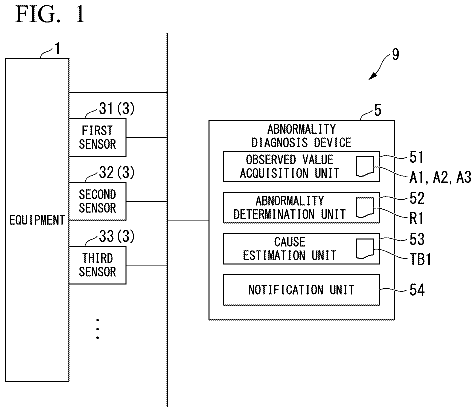
As shown in FIG. 1 , a facility 9 includes equipment 1 , an abnormality diagnosis device 5 , and a first observation system 3 .

The equipment 1 is, for example, a large refrigerator, a submersible pump, and the like.

The abnormality diagnosis device 5 detects whether or not there is an abnormality in the equipment 1 and diagnoses the cause of the abnormality. Also, the abnormality diagnosis device 5 is connected to the first observation system 3 by wire or wireless communication.

The first observation system 3 is a system for observing the state of the equipment 1 and includes, for example, a plurality of sensors (a first sensor 31 , a second sensor 32 , a third sensor 33 , and the like).

The first sensor 31 may be, for example, a pressure sensor provided inside of the equipment 1 and configured to measure the internal pressure of the equipment 1 as an observed value A 1 . The second sensor 32 may be, for example, a thermometer provided at an inlet or an outlet of the equipment 1 and configured to measure an inlet temperature or an outlet temperature of the equipment 1 as an observed value A 2 . The third sensor 33 may be, for example, a flowmeter provided in the equipment 1 and configured to measure a flow rate of a liquid, gas, or the like flowing through the equipment 1 as an observed value A 3 . The observed values A 1 , A 2 , and A 3 , and the like are examples of state quantities of the equipment 1 in the present embodiment.

(Functional Configuration of Abnormality Diagnosis Device)

The abnormality diagnosis device 5 is a device for detecting whether or not there is an abnormality in the equipment 1 and estimating the cause of the abnormality. As shown in FIG. 1 , the abnormality diagnosis device 5 includes an observed value acquisition unit 51 , an abnormality determination unit 52 , and a cause estimation unit 53 .

The observed value acquisition unit 51 acquires the observed values A 1 , A 2 , and A 3 observed by the first observation system 3 of the equipment 1 as the state quantities of the equipment 1 .

The abnormality determination unit 52 determines whether or not there is an abnormality for each state quantity acquired from the equipment 1 . In the present embodiment, the abnormality determination unit 52 determines that the observed values A 1 , A 2 , and A 3 acquired by the observed value acquisition unit 51 are normal if they are within a constraint R 1 and abnormal if they are outside of the constraint R 1 .

The cause estimation unit 53 estimates a cause of an abnormality in the equipment 1 from a state quantity determined to be abnormal by the abnormality determination unit 52 using a cause correspondence table TB 1 in which the cause of an abnormal mode of the equipment 1 identified in fault tree analysis is associated with a state quantity that is abnormal when the cause has occurred.

The notification unit 54 is a display device, an audio output device, or the like for providing a notification of a determination result of the abnormality determination unit 52 and an estimation result of the cause estimation unit 53 . Also, the notification unit 54 may provide a notification of data to a device different from the abnormality diagnosis device 5 , such as a computer, a smartphone, or a tablet, operated by an operator who operates or monitors the equipment 1 .

(Cause Correspondence Table)

FIG. 2 is a first diagram for describing a cause correspondence table according to the first embodiment of the present disclosure.

FIG. 3 is a second diagram for describing a cause correspondence table according to the first embodiment of the present disclosure.

FIG. 4 is a third diagram for describing a cause correspondence table according to the first embodiment of the present disclosure.

In the present embodiment, the cause correspondence table TB 1 is assumed to be pre-created by a designer of the abnormality diagnosis device 5 or the like before the start of the operation of the equipment 1 . A method of creating this cause correspondence table TB 1 will be described with reference to FIGS. 2 to 4 .

First, at the design stage of the abnormality diagnosis device 5 , an operator who designs, develops, or maintains the abnormality diagnosis device 5 performs fault tree analysis of the equipment 1 on the basis of the product knowledge (the knowledge obtained from design, specifications, experience, and the like) of the equipment 1 and decomposes the abnormal mode capable of occurring in the equipment 1 into a plurality of causes as shown in FIG. 2 .

The abnormal mode represents an undesirable failure, an accident, or the like of the equipment 1 . Causes represent events related to the occurrence of the abnormal mode. The causes may be further decomposed into upper causes and lower causes causing the upper causes and arranged in a hierarchical shape. For example, an event that “the pressure of a condenser becomes high pressure and the operation is impossible” may be set as the abnormal mode. At this time, an event such as a “failure of a pressure sensor (the first sensor 31 )” as cause 1 or an event in which a “pressure-specific observed value (the observed value A 1 ) is actually large” as cause 3 may be set. Also, in relation to cause 3 , a “malfunction of a cooling tower,” a “malfunction of a circulation pump,” or the like may be set as lower cause 3 - 1 or 3 - 2 .

Although an example in which only one abnormal mode is set is shown in FIG. 2 , the present disclosure is not limited thereto. In accordance with a configuration and characteristics of the equipment 1 , a plurality of abnormal modes may be set and a tree as shown in FIG. 2 may be configured for each abnormal mode. Although an example in which the causes are decomposed into two layers is shown in FIG. 2 , the present disclosure is not limited thereto. In accordance with the configuration and characteristics of the equipment 1 , the causes may be decomposed into three or more layers.

Also, the operator associates each of the plurality of causes obtained in the fault tree analysis with an observed value that becomes an abnormal value (a value outside of the constraint R 1 ) when this cause has occurred. In the present embodiment, as shown in FIG. 2 , the operator associates the causes with the observed values A 1 , A 2 , and A 3 that can be observed by the first observation system 3 of the equipment 1 . For example, if it is known that the observed value A 1 and the observed value A 3 are abnormal when cause 3 - 1 has occurred from the product knowledge of the equipment 1 , the observed value A 1 and the observed value A 3 are associated with cause 3 - 1 .

When the association between the fault tree analysis result and the observed value is completed, the operator creates a cause correspondence table TB 1 as shown in FIG. 3 . The cause correspondence table TB 1 shows which cause of the abnormal mode can occur for each combination pattern of results of determining the observed values A 1 , A 2 , and A 3 .

For example, as shown in FIG. 4 , it is assumed that only the observed value A 1 of the equipment 1 is determined to be abnormal. In this case, three causes of “cause 1 - 1 ,” “cause 2 ,” and “cause 3 - 1 ” are considered as causes that can occur when the observed value A 1 is abnormal. However, “cause 2 ” and “cause 3 - 1 ” are causes that occur when both observed values A 1 and A 3 are abnormal. In the example of FIG. 4 , because the observed value A 3 is normal, it is excluded from a candidate for the cause. Therefore, in the present example, it is possible to estimate that “cause 1 - 1 (cause 1 )” is a cause that caused the abnormal mode. In this way, the operator creates the cause correspondence table TB 1 shown in FIG. 3 by associating causes that may occur with each combination pattern of the results of determining the observed values A 1 , A 2 , and A 3 .

(Processing Flow of Abnormality Diagnosis Method)

FIG. 5 is a flowchart showing an example of a process of the abnormality diagnosis device according to the first embodiment of the present disclosure.

Hereinafter, details of the abnormality diagnosis process of the abnormality diagnosis device 5 according to the present embodiment will be described with reference to FIG. 5 .

As shown in FIG. 5 , the observed value acquisition unit 51 of the abnormality diagnosis device 5 acquires the observed values A 1 , A 2 , and A 3 from the first sensor 31 , the second sensor 32 , and the third sensor 33 of the equipment 1 (step S 101 ).

Subsequently, the abnormality determination unit 52 of the abnormality diagnosis device 5 determines whether or not there is an abnormality for each of the observed values A 1 , A 2 , and A 3 (step S 102 ).

Subsequently, the cause estimation unit 53 of the abnormality diagnosis device 5 determines whether or not there is an observed value determined to be abnormal (step S 103 ).

For example, the abnormality determination unit 52 determines that the observed value A 1 is normal when the observed value A 1 is less than or equal to a threshold value (an upper limit value or a lower limit value) set as the constraint R 1 . On the other hand, the abnormality determination unit 52 determines that the observed value A 1 is abnormal when the observed value A 1 exceeds the threshold value.

Also, the abnormality determination unit 52 may determine that the observed value A 1 is normal when an amount of change in the observed value A 1 is less than or equal to the threshold value set as the constraint R 1 . In this case, the abnormality determination unit 52 determines that the observed value A 1 is abnormal when the amount of change in the observed value A 1 exceeds the threshold value.

Furthermore, the abnormality determination unit 52 may determine whether the observed value A 1 indicates a normal pattern within the constraint R 1 or indicates an abnormal pattern outside of the constraint R 1 using a known abnormality detection algorithm using a k-nearest neighbor algorithm, a one class support vector machine (SVM), or the like.

The abnormality determination unit 52 determines whether the observed values A 2 and A 3 are normal or abnormal, respectively.

Subsequently, the abnormality determination unit 52 determines whether or not all observed values were normal (step S 103 ).

When the abnormality determination unit 52 determines that all observed values A 1 , A 2 , and A 3 are normal (step S 103 : YES), the abnormality determination unit 52 determines that the operating state of the equipment 1 is normal (step S 104 ).

On the other hand, when the abnormality determination unit 52 determines that at least one of the observed values A 1 , A 2 , and A 3 is abnormal (step S 103 : NO), it is determined that the operating state of the equipment 1 is abnormal (an abnormal mode has occurred). In this case, the cause estimation unit 53 estimates the cause of the abnormal mode on the basis of the cause correspondence table TB 1 ( FIG. 3 ) (step S 105 ).

Specifically, the cause estimation unit 53 selects a cause associated with a combination pattern of an observed value determination result of the abnormality determination unit 52 from the cause correspondence table TB 1 . For example, as in the example of FIG. 4 , it is assumed that a result of determining the observed value A 1 is “abnormal” and results of determining the observed values A 2 and A 3 are “normal.” In this case, the cause estimation unit 53 estimates that “cause 1 - 1 ” associated with “pattern 4” indicating a determination result combination is a cause of the abnormal mode of the equipment 1 with reference to the cause correspondence table TB 1 .

Also, as shown in “pattern 5” of FIG. 3 , there may be a pattern in which the causes cannot be narrowed down to one. In this case, the cause estimation unit 53 may estimate both “cause 2 ” and “cause 3 - 1 ” corresponding to “pattern 5” as candidates for the cause of the abnormal mode without identifying only one cause of the abnormal mode.

Also, in relation to “pattern 5” in which the causes cannot be narrowed down to one from the cause correspondence table TB 1 , for example, an additional observation system (not shown) for identifying “cause 2 ” and “cause 3 - 1 ” may be provided in the equipment 1 in another embodiment. In this case, the cause estimation unit 53 may further estimate whether the cause of the abnormal mode when “pattern 5” is observed is “cause 2 ” or “cause 3 - 1 ” on the basis of the observed value obtained from this additional observation system. At this time, it is only necessary to provide the additional observation system only at locations corresponding to causes that cannot be identified only by the observed values of the first observation system 3 , such as “cause 2 ” and “cause 3 - 1 ” of “pattern 5.” Therefore, it is not necessary to provide an additional observation system for causes that can be narrowed down to one from the observed values of the first observation system 3 . Thus, even if an additional observation system is provided for identifying the causes, the increase in the number of observation systems can be minimized.

In yet another embodiment, the cause estimation unit 53 may further estimate whether the cause of the abnormal mode when “pattern 5” is observed is “cause 2 ” or “cause 3 - 1 ” by further executing an inspection procedure for narrowing down the causes. Thereby, because an additional observation system for identifying causes is not required, the cost related to the diagnosis of an abnormality in the equipment 1 can be suppressed.

Subsequently, the notification unit 54 provides a notification of the determination result of the abnormality determination unit 52 (step S 106 ). Also, when the operating state of the equipment 1 is determined to be abnormal by the abnormality determination unit 52 , the notification unit 54 further provides a notification of a cause estimated by the cause estimation unit 53 .

The abnormality diagnosis device 5 detects whether or not there is an abnormality in the equipment 1 in real time by iteratively executing a series of processing steps shown in FIG. 5 during the operation of the equipment 1 and estimates the cause of the abnormality when an abnormality occurs.

Operation and Effects

As described above, in the abnormality diagnosis device 5 according to the present embodiment, when the abnormality determination unit 52 detects at least one abnormality among state quantities (the observed values A 1 , A 2 , and A 3 ) acquired from the equipment 1 , the cause estimation unit 53 estimates the cause of the abnormal mode of the equipment 1 on the basis of the cause correspondence table TB 1 in which the cause of the abnormal mode is pre-associated with the state quantity that is abnormal when the cause has occurred.

Thereby, the abnormality diagnosis device 5 can easily and accurately estimate the cause of the abnormality in the equipment 1 on the basis of the cause correspondence table TB 1 .

Second Embodiment

Subsequently, the abnormality diagnosis device 5 according to the second embodiment of the present disclosure will be described. Components that are the same as those of the first embodiment are denoted by the same reference signs and detailed description thereof will be omitted.

(Cause Correspondence Table)

FIG. 6 is a first diagram for describing a cause correspondence table according to a second embodiment of the present disclosure.

FIG. 7 is a second diagram for describing a cause correspondence table according to the second embodiment of the present disclosure.

FIG. 8 is a third diagram for describing a cause correspondence table according to the second embodiment of the present disclosure.

In the present embodiment, it is assumed that a cause correspondence table TB 2 is pre-created by the designer of the abnormality diagnosis device 5 or the like before the start of operation of the equipment 1 . A method of creating a cause correspondence table TB 2 according to the present embodiment will be described with reference to FIGS. 6 to 8 .

First, as shown in FIG. 6 , at the design stage of the abnormality diagnosis device 5 , an operator who designs, develops, or maintains the abnormality diagnosis device 5 performs fault tree analysis of the equipment 1 . This is similar to the first embodiment. Also, in the present embodiment, an abnormality degree for a possible value of each of the observed values A 1 , A 2 , and A 3 when this cause occurs is associated with each of the plurality of causes obtained in the fault tree analysis.

The abnormality degree is an evaluation value obtained by discretizing each observed value into a plurality of levels in accordance with a difference from the constraint R 1 set for each observed value. For example, the abnormality degree may be discretized as any one of two to seven levels for each observed value as shown in the discretization table of FIG. 7 . For example, in the case of discretization into three levels, the abnormality degree is expressed by three levels: “negative” in which the observed value is a value at the negative side of the constraint R 1 , “normal” in which the observed value is within the constraint R 1 , and “positive” in which the observed value is a value at the positive side of the constraint R 2 . Also, in the case of discretization into five levels, for example, in accordance with how negative/positive the observed value is from the constraint R 1 , “negative”/“positive” may be further divided into two levels of “high negative”/“high positive” and “low negative”/“low positive.” In the case of discretization into seven levels, for example, in accordance with how negative/positive the observed value is from the constraint R 1 , “negative”/“positive” may be further divided into three levels of “high negative”/“high positive,” “medium negative”/“medium positive,” and “low negative”/“low positive.”

In the present embodiment, for example, when it is difficult to narrow down the causes to one with only two abnormality levels (“normal” or “abnormal”) (for example, “pattern 5” in the cause correspondence table TB 1 of FIG. 3 ), the abnormality degree in the observed value is subdivided into three to seven levels. The discretization level may differ according to each observed value. In the present embodiment, as shown in FIG. 6 , an example in which each observed value is represented by five abnormality levels will be described.

When the association between the fault tree analysis result and the abnormality degree in the observed value is completed, the operator creates a cause correspondence table TB 2 as shown in FIG. 8 . The cause correspondence table TB 2 shows which cause of the abnormal mode can occur for each combination pattern of the abnormality degrees in the observed values A 1 , A 2 , and A 3 .

(Processing Flow of Abnormality Diagnosis Method)

FIG. 9 is a flowchart showing an example of a process of the abnormality diagnosis device according to the second embodiment of the present disclosure.

Hereinafter, details of the abnormality diagnosis process of the abnormality diagnosis device 5 according to the present embodiment will be described with reference to FIG. 9 .

As shown in FIG. 9 , the observed value acquisition unit 51 of the abnormality diagnosis device 5 acquires the observed values A 1 , A 2 , and A 3 from the first sensor 31 , the second sensor 32 , and the third sensor 33 of the equipment 1 (step S 111 ).

Subsequently, the abnormality determination unit 52 of the abnormality diagnosis device 5 determines an abnormality degree corresponding to a difference of each of the observed values A 1 , A 2 , and A 3 from the constraint R 1 set for each observed value (step S 112 ).

For example, the abnormality determination unit 52 determines that the observed value A 1 is one of five abnormality levels of “high negative,” “low negative,” “normal,” “low positive,” and “high positive.” The abnormality determination unit 52 determines that the observed value A 1 is normal, for example, when the observed value A 1 is within a range of a first lower limit value or more and less than a first upper limit value set as the constraint R 1 . Also, the abnormality determination unit 52 determines that the abnormality level in the observed value A 1 is “low negative” when the observed value A 1 is less than the first lower limit value and greater than or equal to the second lower limit value and determines that the abnormality level in the observed value A 1 is “high negative” when the observed value A 1 is less than the second lower limit value. The abnormality determination unit 52 determines that the abnormality level in the observed value A 1 is “low positive” when the observed value A 1 is greater than or equal to the first upper limit value and less than the second upper limit value and determines that the abnormality level in the observed value A 1 is “high positive” when the observed value A 1 is greater than or equal to the second upper limit value.

Also, in other embodiments, the abnormality determination unit 52 may determine the abnormality degree on the basis of an amount of change in the observed value A 1 or may determine an abnormality degree in the observed value A 1 using a known abnormality detection algorithm using a k-nearest neighbor algorithm, a one class SVM, or the like.

Also, the abnormality determination unit 52 similarly determines the abnormality degree for the observed values A 2 and A 3 .

Subsequently, the abnormality determination unit 52 determines whether or not abnormality degrees in all observed values are normal (step S 113 ).

When the abnormality determination unit 52 determines that the abnormality degrees in all observed values A 1 , A 2 , and A 3 are normal (step S 113 : YES), the abnormality determination unit 52 determines that the operating state of the equipment 1 is normal (step S 114 ).

On the other hand, when it is determined that at least one of the abnormality levels of the observed values A 1 , A 2 , and A 3 is a level other than the normal level (any one of a high negative level, a low negative level, a low positive level, and a high positive level) (step S 113 : NO), the abnormality determination unit 52 determines that the operating state of the equipment 1 is abnormal (an abnormal mode has occurred). In this case, the cause estimation unit 53 estimates the cause of the abnormal mode on the basis of the cause correspondence table TB 2 ( FIG. 8 ) (step S 115 ).

Specifically, the cause estimation unit 53 selects a cause associated with a combination pattern of abnormality degrees in observed values by the abnormality determination unit 52 from the cause correspondence table TB 2 . For example, as in the example of FIG. 8 , it is assumed that the abnormality degree in the observed value A 1 is “low positive,” the abnormality degree in the observed value A 2 is “normal,” and the abnormality degree in the observed value A 3 is “low negative.” In this case, the cause estimation unit 53 estimates that “cause 2 ” associated with “pattern 2” indicating a combination of the determination results is the cause of the abnormal mode of the equipment 1 with reference to the cause correspondence table TB 2 .

Subsequently, the notification unit 54 provides a notification of the determination result of the abnormality determination unit 52 (step S 116 ). Also, when the operating state of the equipment 1 is determined to be abnormal by the abnormality determination unit 52 , the notification unit 54 further provides a notification of the cause estimated by the cause estimation unit 53 .

The abnormality diagnosis device 5 detects whether or not there is an abnormality in the equipment 1 in real time by iteratively executing the series of processing steps shown in FIG. 9 during the operation of the equipment 1 and estimates the cause of the abnormality when the abnormality occurs.

Operation and Effects

As described above, in the abnormality diagnosis device 5 according to the present embodiment, the abnormality determination unit 52 further determines the abnormality degree with respect to each state quantity in accordance with the difference of each observed value from the constraint R 1 . The cause estimation unit 53 estimates the cause of the abnormal mode of the equipment 1 using the cause correspondence table TB 2 in which the cause of the abnormal mode is pre-associated with the abnormality degree for each observed value.

For example, in the first embodiment, it may be difficult to narrow down the causes of the abnormal mode to one from the determination result (two levels) indicating whether or not there is an abnormality in the observed value. However, the abnormality diagnosis device 5 according to the present embodiment can narrow down the causes more finely by making a determination after subdividing each observed value into a large number of abnormality levels instead of two levels of “normal” and “abnormal.”

Third Embodiment

Next, the abnormality diagnosis device 5 according to the third embodiment of the present disclosure will be described. Components that are the same as those of the first and second embodiments are denoted by the same reference signs and detailed description thereof will be omitted.

(Functional Configuration of Abnormality Diagnosis Device)

FIG. 10 is a diagram showing a functional configuration of an abnormality diagnosis device according to the third embodiment of the present disclosure.

As shown in FIG. 10 , the abnormality diagnosis device 5 according to the present embodiment further includes an estimate acquisition unit 55 .

The estimate acquisition unit 55 acquires physical quantity estimates PV 1 and PV 2 and the like of the equipment 1 estimated on the basis of the observed values A 1 , A 2 , and A 3 acquired by the observed value acquisition unit 51 as state quantities of the equipment 1 . Also, in the present embodiment, the physical quantity estimate PV is an internal state quantity of the equipment 1 that cannot be observed by the observation system that affects a relationship between input and output conditions of the equipment 1 . The physical quantity estimate PV is, for example, a work quantity within the equipment 1 such as a terminal temperature difference or a refrigerating capacity of a heat exchanger provided in the equipment 1 or the like.

(Cause Correspondence Table)

FIG. 11 is a first diagram for describing a cause correspondence table according to the third embodiment of the present disclosure.

FIG. 12 is a second diagram for describing the cause correspondence table according to the third embodiment of the present disclosure.

A cause correspondence table TB 3 is assumed to be pre-created by a designer of the abnormality diagnosis device 5 or the like before the start of operation of the equipment 1 in the present embodiment as well. A method of creating the cause correspondence table TB 3 according to the present embodiment will be described with reference to FIGS. 11 and 12 .

First, as shown in FIG. 11 , at the design stage of the abnormality diagnosis device 5 , an operator who designs, develops, or maintains the abnormality diagnosis device 5 performs fault tree analysis of the equipment 1 . This is similar to the first and second embodiments. Also, in the present embodiment, an abnormality degree for a possible value of each of the physical quantity estimate PV 1 , the physical quantity estimate PV 2 , the observed value A 1 , and the like is associated with each of the plurality of causes obtained in the fault tree analysis. Although an example in which the physical quantity estimates PV 1 and PV 2 and the state quantity A 1 are classified according to five abnormality levels in FIG. 11 , the present disclosure is not limited thereto. As long as it is possible to narrow down the causes of the abnormal mode to one, an abnormality degree in each of the physical quantity and the observed value may be set to any one of two to seven levels shown in FIG. 7 .

When the association between the fault tree analysis result and the abnormality degree in the physical quantity and the observed value is completed, the operator creates the cause correspondence table TB 3 as shown in FIG. 12 . The cause correspondence table TB 3 shows which cause of the abnormal mode can occur for each combination pattern of abnormality degrees in the physical quantity estimate PV 1 , the physical quantity estimate PV 2 , and the observed value A 1 .

(Processing Flow of Abnormality Diagnosis Method)

FIG. 13 is a flowchart showing an example of a process of the abnormality diagnosis device according to the third embodiment of the present disclosure.

Hereinafter, details of the abnormality diagnosis process of the abnormality diagnosis device 5 according to the present embodiment will be described with reference to FIG. 13 .

As shown in FIG. 13 , the observed value acquisition unit 51 of the abnormality diagnosis device 5 acquires the observed values A 1 , A 2 , and A 3 from the first sensor 31 , the second sensor 32 , and the third sensor 33 of the equipment 1 (step S 121 ).

Subsequently, the estimate acquisition unit 55 of the abnormality diagnosis device 5 acquires the physical quantity estimates PV 1 and PV 2 of the equipment 1 estimated on the basis of the observed values A 1 , A 2 , and A 3 (step S 122 ). For example, the estimate acquisition unit 55 estimates and acquires the physical quantity estimates PV 1 and PV 2 of the equipment 1 using a known estimation algorithm using a Kalman filter, a hidden Markov model, or the like.

Subsequently, the abnormality determination unit 52 of the abnormality diagnosis device 5 determines whether or not there is an abnormality or the abnormality degree for each of the observed value A 1 acquired by the observed value acquisition unit 51 and the physical quantity estimates PV 1 and PV 2 estimated by the estimate acquisition unit 55 (step S 123 ). Content of the specific processing is similar to step S 102 ( FIG. 5 ) of the first embodiment or step S 112 ( FIG. 9 ) of the second embodiment.

Subsequently, the abnormality determination unit 52 determines whether or not all observed values and physical quantities are normal (step S 124 ).

When it is determined that all of the observed values A 1 and the physical quantity estimates PV 1 and PV 2 are normal (step S 124 : YES), the abnormality determination unit 52 determines that the operating state of the equipment 1 is normal (step S 125 ).

On the other hand, when it is determined that at least one of the abnormality levels of the observed value A 1 and the physical quantity estimates PV 1 and PV 2 is a level other than the normal level (any one of an abnormal level, a high negative level, a low negative level, a low positive level, and a high positive level) (step S 124 : NO), the abnormality determination unit 52 determines that the operating state of the equipment 1 is abnormal (an abnormal mode has occurred). In this case, the cause estimation unit 53 estimates the cause of the abnormal mode on the basis of the cause correspondence table TB 3 ( FIG. 12 ) (step S 126 ). Content of the specific processing is similar to step S 105 ( FIG. 5 ) of the first embodiment and step S 115 ( FIG. 9 ) of the second embodiment.

Subsequently, the notification unit 54 provides a notification of the determination result by the abnormality determination unit 52 (step S 127 ). Also, when the operating state of the equipment 1 is determined to be abnormal by the abnormality determination unit 52 , the notification unit 54 further provides a notification of a cause estimated by the cause estimation unit 53 .

The abnormality diagnosis device 5 detects whether or not there is an abnormality in the equipment 1 in real time and estimates the cause of the abnormality when an abnormality occurs by iteratively executing the series of processing steps shown in FIG. 13 during the operation of the equipment 1 .

Operation and Effects

As described above, the abnormality diagnosis device 5 according to the present embodiment further includes the estimate acquisition unit 55 configured to estimate the physical quantity estimates PV 1 and PV 2 of the equipment 1 that cannot be observed by the first observation system 3 .

Thereby, the abnormality diagnosis device 5 can perform the determination of whether or not there is an abnormality and the estimation of a cause of the abnormality using the physical quantity estimates PV 1 and PV 2 obtained by estimating the internal state quantity of the equipment 1 in addition to the observed value A 1 acquired from the first observation system 3 of the equipment 1 . Thereby, the abnormality diagnosis device 5 can improve the accuracy of detection even in an abnormal mode whose detection is difficult only from changing in the observed value.

Fourth Embodiment

Next, the abnormality diagnosis device 5 according to a fourth embodiment of the present disclosure will be described. Components that are the same as those of the first to third embodiments are denoted by the same reference signs and detailed description thereof will be omitted.

FIG. 14 is a diagram showing an overall configuration of a facility according to the fourth embodiment of the present disclosure.

As shown in FIG. 14 , a facility 9 according to the present embodiment further includes an estimation device 2 . Also, the facility 9 according to the present embodiment further includes a second observation system 4 in addition to a first observation system 3 .

(Configuration of First Observation System)

The first observation system 3 is a system for observing a state of equipment 1 .

The first observation system 3 observes a first observed value OB 1 .

For example, the first observation system 3 may be provided in the equipment 1 .

For example, the first observation system 3 may include a first sensor 31 .

For example, the first observation system 3 may observe an observed value A 1 as the first observed value OB 1 .

For example, the first sensor 31 may be provided inside of, for example, the equipment 1 . At this time, the first sensor 31 may be a pressure sensor that measures the internal pressure of the equipment 1 as the observed value A 1 .

(Configuration of Second Observation System)

The second observation system 4 is a system for observing the state of the equipment 1 .

The second observation system 4 observes a second observed value OB 2 .

The second observation system 4 is another observation system that is independent of the first observation system 3 .

For example, the second observation system 4 may be provided in the equipment 1 .

For example, the second observation system 4 may include a second sensor 41 , a third sensor 42 , and a fourth sensor 43 .

For example, the second observation system 4 may observe observed values A 2 , A 3 , and A 4 as the second observed value OB 2 .

For example, the second sensor 41 may be provided at, for example, an outlet of the equipment 1 . At this time, the second sensor 41 may be a thermometer that measures an outlet temperature, which is the temperature of a fluid such as a liquid or gas outgoing from the inside of the equipment 1 , as the observed value A 2 .

Also, the third sensor 42 may be provided at, for example, an inlet of the equipment 1 , for example. At this time, the third sensor 42 may be a thermometer that measures an inlet temperature, which is the temperature of a fluid such as a liquid or gas incoming into the equipment 1 , as the observed value A 3 .

Also, the fourth sensor 43 may be provided in, for example, the equipment 1 . At this time, the fourth sensor 43 may be a flowmeter that measures the flow rate of a fluid such as a liquid or gas flowing through the equipment 1 as the observed value A 4 .

(Configuration of Estimation Device)

The estimation device 2 is a device for estimating a parameter PR of each model of the equipment 1 , the first observation system 3 , and the second observation system 4 .

Also, the estimation device 2 is a device for providing a network model NWM including the estimated parameter PR to the abnormality diagnosis device 5 .

The estimation device 2 includes an observation system constraint determination unit 22 , a model estimation unit 23 , and a consistency determination unit 24 .

For example, the estimation device 2 may further include a physical quantity constraint determination unit 25 and a model constraint determination unit 26 .

Also, the estimation device 2 may further include an acquisition unit 21 and an output unit 27 .

(Composition of Acquisition Unit)

The acquisition unit 21 acquires the first observed value OB 1 .

For example, the acquisition unit 21 may acquire the observed value A 1 from the first observation system 3 as the first observed value OB 1 .

For example, the acquisition unit 21 may acquire the internal pressure of the equipment 1 measured by the first sensor 31 as the observed value A 1 .

The acquisition unit 21 acquires the second observed value OB 2 .

For example, the acquisition unit 21 may acquire the observed values A 2 , A 3 , and A 4 from the second observation system 4 as the second observed value OB 2 .

For example, the acquisition unit 21 may acquire the outlet temperature measured by the second sensor 41 as the observed value A 2 .

For example, the acquisition unit 21 may acquire the inlet temperature measured by the third sensor 42 as the observed value A 3 .

For example, the acquisition unit 21 may acquire the flow rate measured by the fourth sensor 43 as the observed value A 4 .

(Configuration of Observation System Constraint Determination Unit)

The observation system constraint determination unit 22 determines data DT 2 within the constraint that is data within a first constraint R 1 from time-series data DT 1 of observed values of the first observed value OB 1 observed in the first observation system 3 and the second observed value OB 2 observed in the second observation system 4 .

By determining the consistency of a separate item of each observation system with a constraint condition, the observation system constraint determination unit 22 determines whether or not each observed value is data associated with abnormal behavior as a separate item.

For example, as shown in FIG. 2 , the observation system constraint determination unit 22 may determine data DT 2 inside of a constraint according to an observation system constraint such as a constraint related to a maximum value and a minimum value, a constraint related to a moving average change rate, a constraint related to a spike generation frequency, or a constraint related to a variance within the time window as the first constraint R 1 .

Thereby, the observation system constraint determination unit 22 determines that a record of each observed value including an abnormal value when viewed alone is abnormal on the basis of a measurement principle (a physical law) of each observation system itself.

For example, in the case of FIG. 15 , within the time-series data DT 1 that is time-series data of observed raw values observed in each observation system, data DT 3 is data whose spike generation frequency of an observed value is greater than a prescribed threshold value or data whose variance of the observed value inside of the time window is greater than a prescribed threshold value, and is determined to be outside of a constraint due to the first constraint R 1 .

Likewise, within the time-series data DT 1 , data DT 4 is data whose observed value is greater than a maximum value prescribed by an upper limit value or data whose observed value is less than a minimum value prescribed by a lower limit value, and is determined to be outside of a constraint due to the first constraint R 1 .

Likewise, within the time-series data DT 1 , data DT 5 is data whose moving average change rate is greater than a prescribed threshold value, and is determined to be outside of a constraint due to the first constraint R 1 .

On the other hand, data that is not outside of the constraint is determined to be data DT 2 within the constraint.

For example, when an out-of-constraint determination has been made in any observation system among the observation systems, the observation system constraint determination unit 22 may make the out-of-constraint determination even with respect to the data of the other observation system at the same time and the estimation device 2 may not perform a subsequent process.

(Composition of Model Estimation Unit)

The model estimation unit 23 estimates parameters PR of a plurality of models including an observation model MLO that is a model of each observation system and a physical model MLP that is a model inside of the equipment 1 in which the observation system is provided on the basis of the data DT 2 within the constraint.

For example, the model estimation unit 23 may include the network model NWM including a plurality of observation models MLO and a plurality of physical models MLP.

For example, each of the plurality of observation models MLO and the plurality of physical models MLP may include a parameter PR.

For example, the model estimation unit 23 may estimate the parameter PR of each of the observation models MLO and the physical models MLP in a network model NWM 1 as shown in FIG. 3 , which is an example of the network model NWM.

As shown in FIG. 16 , in the network model NWM 1 , the model estimation unit 23 can estimate the physical quantity estimate PV 1 , which is one of a plurality of physical quantity estimates PV 1 , from the observed value A 1 via one observation model MLO.

On the other hand, in the network model NWM 1 , the model estimation unit 23 can estimate the physical quantity estimate PV 1 from the observed value A 2 , the observed value A 3 , and the observed value A 4 via the plurality of observation models MLO and the plurality of physical models MLP.

That is, in the network model NWM 1 , the model estimation unit 23 can estimate a common physical quantity estimate PV 1 from different systems.

As shown in FIG. 16 , for example, in the model estimation unit 23 , the parameter PR of the observation model MLO related to the observed value A 2 may be estimated from the observed value A 2 and an observed value A 2 ′ before the step in which the observed value A 2 is observed (an observed value A 2 ′ measured at a point in time immediately before the observed value A 2 is measured).

Likewise, in the model estimation unit 23 , the parameter PR of the observation model MLO related to the observed value A 3 may be estimated from the observed value A 3 and an observed value A 3 ′ before the step in which the observed value A 3 is observed (an observed value A 3 ′ measured at a point in time immediately before the observed value A 3 is measured).

(Configuration of Model)

For example, each of the observation model MLO and the physical model MLP may be expressed in the form of a nonlinear polynomial based on a theoretical formula and an empirical formula. At this time, a coefficient of the polynomial corresponds to the parameter PR and becomes a parameter for expressing a variation in the actual equipment 1 .

Here, the physical model MLP will be described in detail. For example, each physical model MLP may be a model derived from known pure physical laws in physical phenomena.

For example, a physical model MLPA shown in FIG. 16 may be a model in which a physical quantity estimate PVA indicating a work quantity within the equipment 1 such as a refrigerating capacity or the like can be calculated from a physical quantity estimate PV 2 indicating an outlet temperature, a physical quantity estimate PV 3 indicating an inlet temperature, and a physical quantity estimate PV 4 indicating a flow rate.

For example, a physical model MLPB shown in FIG. 16 may be a model in which a physical quantity estimate PVB indicating a saturated temperature inside of the equipment 1 can be calculated from the physical quantity estimate PV 2 indicating the outlet temperature and the physical quantity estimate PVA indicating the work quantity.

For example, a physical model MLPC shown in FIG. 16 may be a model in which a physical quantity estimate PV 1 indicating the pressure (saturated vapor pressure) within the equipment 1 can be calculated from the physical quantity estimate PVB indicating the saturation temperature inside of the equipment 1 .

Next, the observation model MLO will be described in detail.

For example, each observation model MLO may be a representative model as shown in FIG. 17 .

In FIG. 17 , an error from a true value caused due to the characteristics of the sensor is indicated as an internal cause and an error caused due to a cause other than a value of an observation target is indicated as an external cause.

In addition to the internal and external causes that can be modeled, observed values are further affected by random noise components.

Also, it is necessary for the external cause to be assumed to be any one of a “negligibly small” cause, an “external cause measured by another sensor,” and a cause having an “amount of data capable of being handled as noise.”

The accuracy of the observation system is prescribed by a full-scale error (±0% F.S.) shown in FIG. 18 or an indicated value error (±0% R.D.) as shown in FIG. 19 after all errors are taken into account or an index obtained by combining these errors.

Also, these error ranges indicate only the accuracy when the normal operation is performed and deviate from the range when the sensor is misaligned or malfunctioned.

Also, when the same value is continuously measured, a magnitude of a variation in a result of comparing values obtained by taking the time window average is referred to as Allan variance.

Typical Allan variance shows variance as shown in FIG. 20 . Also, σy(f) shown in FIG. 20 is a value related to a magnitude of the Allan variance.

As shown in FIGS. 20 and 21 , while an average time τ is short, the influence of noise is dominant and a variation between the average values gradually decreases. However, when the average time τ is extended, the influence of long-term fluctuations in the observation system parameters becomes apparent and the variation gradually increases.

Therefore, for example, the parameter PR of the observation model MLO may be estimated ideally on the basis of record data in which the Allan variance is only minimized.

For example, the model estimation unit 23 may accumulate sums of squares of average values of physical quantity estimates PV of all systems and errors of the physical quantity estimates PV of the systems in all records with respect the physical quantity estimates PV capable of being estimated from the systems using data of a number of records required to estimate each parameter PR from the most recent observed value within the data DT 2 within the constraint that is not abnormal as an observed value of a separate item in the observation system constraint determination unit 22 . At this time, a reward function for the correctness of the estimation may be determined on the basis of a magnitude of a penalty coefficient predetermined for an accumulated value and a magnitude of a correction term of each parameter PR and the parameter PR may be estimated so that a value thereof is minimized.

For example, the model estimation unit 23 may estimate the parameter PR so that a sum of a penalty for the deviation between the physical quantity estimates PV 1 estimated from the systems and a penalty for the correction term of each parameter PR is minimized with respect to an observation system in which a common physical quantity estimate PV 1 can be derived by converting values based on models of the network model NWM 1 .

Also, even if the number of observation systems is generally extremely small with respect to the number of parameters PR to be estimated, the model estimation unit 23 can estimate the physical quantity estimate PV 1 using a plurality of records.

For example, the observation model MLO may be an observation model in which an appropriate range is simplified in consideration of usage conditions of the equipment 1 and specifications of each sensor instead of a faithfully modeled observation model.

For example, in the observation model MLO related to the observed value A 1 , the penalty for the correction term from the ideal state of a bias or scale factor (hereinafter also referred to as “SF”) may be determined on the basis of the accuracy of the sensor.

The model estimation unit 23 may be configured so that a reward function for a magnitude of a mean squared error of differences of the physical quantity estimates PV 1 from an average value of a plurality of physical quantity estimates PV 1 is determined as deviation between physical quantity estimates estimated from the systems in the network model NWM 1 .

For example, as shown in FIG. 22 , when each physical quantity estimate PV can be estimated from three or more different systems in the network model NWM including the plurality of models, the model estimation unit 23 may determine a reward function for a magnitude of a mean squared error of differences of physical quantity estimates PV from an average value of a plurality of physical quantity estimates PV as the deviation between the physical quantity estimates PV estimated from the three or more systems.

Likewise, in the case shown in FIG. 22 , the model estimation unit 23 may estimate the parameter PR so that a sum of the penalty for the deviation between the physical quantity estimates PV estimated from the three or more systems and the penalty for the correction term of each parameter PR is minimized.

(Configuration of Consistency Determination Unit)

The consistency determination unit 24 determines the consistency of the model from deviation between the first observed value OB 1 and the first predicted observed value PA 1 predicted from the second observed value OB 2 on the basis of parameters PR of the plurality of models estimated by the model estimation unit 23 .

Thereby, the consistency determination unit 24 can cause a certain observed value from another observed value to regress on the basis of the estimated parameter PR and evaluate a magnitude of the deviation.

Here, the first predicted observed value PA 1 is a value derived by value conversion based on each model of the network model NWM 1 and is a value corresponding to the first observed value OB 1 in the network model NWM 1 .

For example, the consistency determination unit 24 may compare the first predicted observed value PA 1 , which is a regression result predicted on the basis of the parameter PR of each model estimated by the model estimation unit 23 , with the first observed value OB 1 , which is an actually measured value.

For example, as the model consistency, the consistency determination unit 24 may determine whether the deviation between the first predicted observed value PA 1 predicted from the second observed value OB 2 and the first observed value OB 1 is within a specification range of the first observation system 3 .

For example, as shown in FIG. 23 , as the model consistency, the consistency determination unit 24 may determine whether deviation between the observed value A 1 and the first predicted observed value PA 1 predicted from the observed value A 2 , the observed value A 3 , and the observed value A 4 is within a specification range of the first observation system 3 .

For example, the consistency determination unit 24 may predict the first predicted observed value PA 1 from the observed value A 2 , the observed value A 3 , and the observed value A 4 via the plurality of observation models MLO and the plurality of physical models MLP in which the parameter PR estimated by the model estimation unit 23 is introduced and compare the first predicted observed value PA 1 , which has been predicted, with the observed value A 1 .

For example, the consistency determination unit 24 may acquire a difference between the first predicted observed value PA 1 and the first observed value OB 1 as the deviation between the first predicted observed value PA 1 and the first observed value OB 1 . At this time, as a model consistency determination, the consistency determination unit 24 may determine that the plurality of observation models MLO and plurality of physical models MLP in which the parameter PR is introduced are consistent if the acquired difference is less than or equal to a prescribed threshold value.

For example, the consistency determination unit 24 may perform mutual regression and evaluate mutual consistency for all observation systems.

For example, in addition to the evaluation shown in FIG. 23 , as shown in FIG. 24 , the consistency determination unit 24 may predict the second predicted observation value PA 2 from the observed value A 1 , the observed value A 3 and the observed value A 4 via the plurality of observation models MLO and plurality of physical models MLP into which the parameter PR estimated by the model estimation unit 23 is introduced and may further compare the predicted second predicted observation value PA 2 with the observed value A 2 .

Furthermore, as in the evaluation related to the observed value A 1 shown in FIG. 23 and the evaluation related to the observed value A 2 shown in FIG. 24 , the consistency determination unit 24 may perform an evaluation process related to the observed value A 3 on the basis of the observed value A 1 , the observed value A 2 , and the observed value A 4 or may perform an evaluation process related to the observed value A 4 on the basis of the observed value A 1 , the observed value A 2 , and the observed value A 3 .

For example, as shown in FIGS. 25 and 26 , when there are a plurality of independent systems for causing the same observed value to regress, the consistency determination unit 24 may obtain deviation for each system associated with the regression and use a minimum value of a plurality of deviations that have been obtained as an observed value evaluation result.

(Configuration of Physical Quantity Constraint Determination Unit)

The physical quantity constraint determination unit 25 determines whether or not the physical quantity estimate PV estimated on the basis of the parameter PR is within a second constraint R 2 .

Here, the physical quantity estimate PV is a physical quantity in the equipment 1 estimated by the physical model MLP.

For example, the physical quantity constraint determination unit 25 may determine whether or not the physical quantity estimate PV estimated on the basis of the parameter PR when the consistency determination unit 24 determines that the models are consistent and the observed value of the data DT 2 within the constraint is within the second constraint R 2 .

For example, the second constraint R 2 may be a prescribed numerical range indicating a physical quantity that is less than or equal to the design level (specification) of the equipment 1 .

For example, the physical quantity constraint determination unit 25 may determine that the physical quantity estimate PV is normal if it is within the second constraint R 2 and that the physical quantity estimate PV is abnormal if it is not within the second constraint R 2 . When the physical quantity estimate PV is determined to be normal, the parameter PR introduced in each model can be regarded as appropriate in the determination of the physical quantity constraint determination unit 25 .

For example, when the physical quantity estimate PV is determined to be abnormal, the physical quantity constraint determination unit 25 may determine that the equipment 1 is abnormal.

That is, it is possible to determine that the equipment 1 is abnormal if the physical quantity estimate PV, which is a physical quantity, does not fall within the constraint of the design specification on the basis of the assumption that a physical quantity can be estimated for the data DT 2 within the constraint, which is a record determined to be normal.

For example, when each observed value of the data DT 2 within the constraint is time-discrete due to the application of the first constraint R 1 , the physical quantity constraint determination unit 25 may perform a time interpolation process for observed values that are discrete and may estimate the physical quantity estimate PV on the basis of the observed value corrected in time.

For example, the physical quantity constraint determination unit 25 may determine whether or not the physical quantity estimate PV estimated at each time step is within the second constraint R 2 .

For example, the physical quantity constraint determination unit 25 may compare each estimated physical quantity estimate PV with the design level (specification) and may convert the estimated physical quantity estimate PV into discrete data of about two to seven levels by determining that it is within the specification, is greater than or equal to the specification, or is less than or equal to the specification.

(Configuration of Model Constraint Determination Unit)

The model constraint determination unit 26 determines whether or not each parameter PR is inside of a third constraint R 3 .

For example, the model constraint determination unit 26 may determine whether or not each parameter PR when the models are determined to be consistent in the consistency determination unit 24 is within the third constraint R 3 .

For example, the third constraint R 3 for each parameter PR in the physical model MLP may be a prescribed numerical range indicating a parameter less than or equal to the design level (specification) of the equipment 1 .

For example, the third constraint R 3 for each parameter PR in the observation model MLO may be a prescribed numerical range indicating the parameter within the design level (specification) of each observed value.

For example, the model constraint determination unit 26 may determine that each parameter PR is normal if it is within the third constraint R 3 or may determine that each parameter PR is abnormal if it is not within the third constraint R 3 . When each parameter PR is determined to be normal, the parameter PR introduced in each model can be regarded as appropriate in the determination process of the model constraint determination unit 26 .

For example, each parameter PR determined by the model constraint determination unit 26 may be a parameter estimated for each batch window or each moving window that has undergone mutual regression.

For example, the model constraint determination unit 26 may compare each estimated parameter PR with the design level (specification) and may convert the estimated parameter PR into discrete data of about two to seven levels by determining that it is within the specification, is greater than or equal to the specification, or is less than or equal to the specification.

For example, when the parameter PR of the physical model MLP is determined to be abnormal, the model constraint determination unit 26 may determine that the equipment 1 is abnormal.

That is, it is possible to determine that the equipment 1 is abnormal if the parameter PR of the physical model MLP does not fall within the constraint of the design specification on the basis of the assumption that parameter estimation is performed correctly.

For example, when the parameter PR of the observation model MLO is determined to be abnormal, the model constraint determination unit 26 may determine that the observation system is abnormal. Furthermore, the model constraint determination unit 26 may determine that a sensor related to the observation model MLO having the parameter PR determined to be abnormal is abnormal. That is, it is possible to determine that the observation system is abnormal if the parameter PR of the observation model MLO does not fall within the constraint of the design specification on the basis of the assumption that parameter estimation is performed correctly.

(Configuration of Output Unit)

The output unit 27 outputs a parameter PR determined to be normal and a physical quantity estimate PV estimated on the basis of the parameter PR.

Also, the output unit 27 outputs a parameter PR determined to be abnormal and a physical quantity estimate PV estimated on the basis of the parameter PR. For example, when the parameter PR determined to be abnormal is the parameter PR of the observation model MLO, the output unit 27 may output information indicating that the sensor related to the observation model MLO having the parameter PR determined to be abnormal is abnormal.

For example, the output unit 27 may output information indicating that the equipment 1 is abnormal when the parameter PR determined to be abnormal is the parameter PR of the physical model MLP.

(Operation of Estimation Device)

The operation of the estimation device 2 of the present embodiment will be described.

The operation of the estimation device 2 corresponds to the estimation method of the present embodiment.

The operation of the estimation device 2 may be performed, for example, as shown in FIG. 27 .

First, the acquisition unit 21 acquires the first observed value OB 1 observed in the first observation system 3 and the second observed value OB 2 observed in the second observation system 4 (ST 01 : acquisition step).

After the execution of ST 01 , the observation system constraint determination unit 22 determines the data DT 2 within the constraint that is data within the first constraint R 1 from the time-series data DT 1 of observed values of the first observed value OB 1 and the second observed value OB 2 (ST 02 : observation system constraint determination step).

After the execution of ST 02 , the model estimation unit 23 estimates parameters PR of a plurality of models including an observation model MLO that is a model of each observation system and a physical model MLP that is a model within the equipment 1 in which the observation system is provided on the basis of the data DT 2 within the constraint (ST 03 : model estimation step).

After the execution of ST 03 , the consistency determination unit 24 determines model consistency from deviation between the first observed value OB 1 and the first predicted observed value PA 1 predicted from the second observed value OB 2 on the basis of the parameters PR of the plurality of models estimated by the model estimation unit 23 (ST 04 : consistency determination step).

For example, in ST 04 , the consistency determination unit 24 may determine that there is an abnormality in the observation model or the physical model when the deviation is greater than a prescribed value (ST 04 A). At this time, the consistency determination unit 24 may delete records that deviate from the model even if optimized.

For example, after the execution of ST 04 A, the consistency determination unit 24 may determine inconsistent data within the data DT 2 within the constraint and exclude the inconsistent data from the data DT 2 within the constraint as abnormal data (ST 04 B).

For example, after the execution of ST 04 , the physical quantity constraint determination unit 25 may determine whether or not the physical quantity estimate PV estimated on the basis of the parameter PR is within the second constraint R 2 (ST 05 : physical quantity constraint determination step).

For example, in parallel with ST 05 , the model constraint determination unit 26 may determine whether or not each parameter PR is within the third constraint R 3 (ST 06 : model constraint determination step).

For example, after the execution of ST 04 and ST 05 , the output unit 27 may output a parameter PR determined to be normal and a physical quantity estimate PV estimated on the basis of the parameter PR and may output a parameter PR determined to be abnormal and a physical quantity estimate PV estimated on the basis of the parameter PR (ST 07 : output step).

(Function of Abnormality Diagnosis Device)

The abnormality diagnosis device 5 according to the present embodiment is different from the third embodiment in that the estimate acquisition unit 55 acquires the physical quantity estimate PV of the equipment 1 from the estimation device 2 . That is, the estimate acquisition unit 55 of the abnormality diagnosis device 5 according to the present embodiment acquires the physical quantity estimate PV estimated by the estimation device 2 as the state quantity of the equipment 1 in step S 122 of FIG. 13 .

Also, the abnormality determination unit 52 of the abnormality diagnosis device 5 according to the present embodiment may further determine whether or not there is an abnormality in the equipment 1 on the basis of determination results of the observation system constraint determination unit 22 and the physical quantity constraint determination unit 25 of the estimation device 2 . For example, in step S 123 of FIG. 13 , the abnormality determination unit 52 of the abnormality diagnosis device 5 may determine that an observed value is abnormal when there is data (an observed value) determined to be outside of the first constraint R 1 by the observation system constraint determination unit 22 of the estimation device 2 . Likewise, in step S 123 of FIG. 13 , the abnormality determination unit 52 of the abnormality diagnosis device 5 may determine that a physical quantity estimate PV is abnormal when there is a physical quantity estimate PV determined to be outside of the second constraint R 2 by the physical quantity constraint determination unit 25 of the estimation device 2 .

Operation and Effects

As described above, in the abnormality diagnosis device 5 according to the present embodiment, the estimate acquisition unit 55 acquires the physical quantity estimate PV of the equipment 1 estimated by the estimation device 2 as the state quantity of the equipment 1 .

Also, because the estimation device 2 according to the present embodiment can estimate and optimize the parameters PR of a plurality of models including the observation model MLO and the physical model MLP, it is possible to estimate a more accurate physical quantity estimate PV.

Thus, the abnormality diagnosis device 5 can further improve the accuracy of estimating the cause of an abnormality using an accurate physical quantity estimate PV.

<Hardware Configuration of Computer>

Also, in each of the above-described embodiments, a program for implementing various types of functions of the abnormality diagnosis device 5 and the estimation device 2 is recorded on a computer-readable recording medium and various types of processing are performed by causing a computer system such as a microcomputer to read and execute the program recorded on the recording medium. Here, the above-described various types of processing are performed by storing the process of the various types of processing of a CPU of a computer system in a computer-readable recording medium in the form of a program and causing the computer to read and execute the program. Also, the computer-readable recording medium is a magnetic disk, a magneto-optical disk, a CD-ROM, a DVD-ROM, a semiconductor memory, or the like. Also, the computer program may be delivered to the computer via a communication circuit and the computer having received the delivered program may execute the program.

In each of the above-described embodiments, an example of a hardware configuration of the computer for executing the program for implementing the various types of functions of the abnormality diagnosis device 5 and the estimation device 2 will be described.

As shown in FIG. 20 , the computer 29 provided in each of the abnormality diagnosis device 5 and the estimation device 2 includes a CPU 291 , a memory 292 , a storage/playback device 293 , an input output interface (hereinafter referred to as an “IO I/F”) 294 , and a communication interface (hereinafter referred to as a “communication I/F”) 295 .

The memory 292 is a medium such as a random-access memory (hereinafter referred to as a “RAM”) temporarily storing data and the like used by a program executed in each of the abnormality diagnosis device 5 and the estimation device 2 .

The storage/playback device 293 is a device for storing data and the like in external media such as a CD-ROM, a DVD, or a flash memory or for reproducing data of external media or the like.

The IO I/F 294 is an interface for inputting/outputting information and the like between the abnormality diagnosis device 5 and the estimation device 2 and other devices.

The communication I/F 295 is an interface that performs communication between the estimation device 2 and another device via a communication circuit such as the Internet or a dedicated communication circuit.

Other Embodiments

While embodiments of the present disclosure have been described above, these embodiments have been presented by way of example only, and are not intended to limit the scope of the disclosure. These embodiments may be embodied in a variety of other forms. Various omissions, substitutions, and changes may be made without departing from the spirit of the disclosure. The disclosure is intended to cover such embodiments or modifications as would fall within the scope and spirit of the disclosure.

APPENDIXES

For example, the abnormality diagnosis device, abnormality diagnosis method, and recording medium storing the program described in the above-described embodiments are ascertained as follows.

(1) According to a first aspect, the abnormality diagnosis device 5 includes the abnormality determination unit 52 configured to determine whether or not there is an abnormality with respect to a state quantity acquired from the equipment 1 ; and the cause estimation unit 53 configured to estimate a cause of the abnormality in the equipment 1 from a state quantity determined to be abnormal by the abnormality determination unit 52 using a cause correspondence table in which a cause of an abnormal mode of the equipment identified in fault tree analysis is associated with the state quantity that is abnormal when the cause has occurred.

Thereby, the abnormality diagnosis device 5 can easily and accurately estimate the cause of the abnormality in the equipment 1 on the basis of the cause correspondence table.

(2) According to a second aspect, the abnormality diagnosis device 5 of the first aspect (1) further includes the observed value acquisition unit 51 configured to acquire an observed value observed by an observation system of the equipment as the state quantity, wherein the abnormality determination unit 52 determines whether or not there is an abnormality in the equipment 1 by comparing the observed value acquired by the observed value acquisition unit 51 with a normal value or a normal pattern of each observed value.

Thereby, the abnormality diagnosis device 5 can easily and accurately estimate the cause of the abnormality using, for example, the observed value observed by the existing observation system of the equipment 1 and the cause correspondence table.

(3) According to a third aspect, in the abnormality diagnosis device 5 of the aspect (1) or (2), the abnormality determination unit 52 further determines an abnormality degree with respect to each state quantity in accordance with a difference from a constraint set for each state quantity and the cause estimation unit 53 estimates the cause of the abnormality in the equipment 1 using the cause correspondence table in which the cause is further associated with the abnormality degree of the state quantity that is abnormal when the cause has occurred.

Thereby, the abnormality diagnosis device 5 can narrow down the causes more finely by subdividing each observed value into a larger number of abnormality levels instead of two levels of “normal” or “abnormal.”

(4) According to a fourth aspect, the abnormality diagnosis device 5 of the aspect (2) further includes the estimate acquisition unit 55 configured to acquire a physical quantity estimate of the equipment 1 estimated on the basis of the observed value acquired by the observed value acquisition unit 51 as the state quantity.

Thereby, the abnormality diagnosis device 5 can perform the determination of whether or not there is an abnormality and the estimation of the cause of the abnormality using the physical quantity estimates PV 1 and PV 2 obtained by estimating the internal state quantity within the equipment 1 in addition to the observed value A 1 acquired from the first observation system 3 of the equipment 1 . Thereby, the abnormality diagnosis device 5 can improve the detection accuracy even in an abnormal mode whose detection is difficult only by changing the observed value.

(5) According to a fifth aspect, there is provided an abnormality diagnosis method including steps of: determining whether or not there is an abnormality with respect to a state quantity acquired from the equipment 1 ; and estimating a cause of the abnormality in the equipment 1 from a state quantity determined to be abnormal using a cause correspondence table in which a cause of an abnormal mode of the equipment 1 identified in fault tree analysis is associated with the state quantity that is abnormal when cause has occurred.

(6) According to a sixth aspect, there is provided a non-transitory computer-readable recording medium storing a program for causing the computer 29 of the abnormality diagnosis device 5 to execute steps of: determining whether or not there is an abnormality with respect to a state quantity acquired from the equipment 1 ; and estimating a cause of the abnormality in the equipment 1 from a state quantity determined to be abnormal using a cause correspondence table in which a cause of an abnormal mode of the equipment 1 identified in fault tree analysis is associated with the state quantity that is abnormal when the cause has occurred.

According to the present disclosure, an abnormality diagnosis device, an abnormality diagnosis method, and a recording medium storing a program can easily and accurately estimate a cause of an abnormality in equipment.

REFERENCE SIGNS LIST

•

• 2 Estimation device • 21 Acquisition unit • 22 Observation system constraint determination unit • 23 Model estimation unit • 24 Consistency determination unit • 25 Physical quantity constraint determination unit • 26 Model constraint determination unit • 27 Output unit • 29 Computer • 3 First observation system • 31 First sensor • 32 Second sensor • 33 Third sensor • 4 Second observation system • 41 Second sensor • 42 Third sensor • 43 Fourth sensor • 5 Abnormality diagnosis device • 51 Observed value acquisition unit • 52 Abnormality determination unit • 53 Cause estimation unit • 54 Notification unit • 55 Estimate acquisition unit